Introduction : Naive look at the output of a digital camera
The goal of this series of articles is to understand how the colours of a digital image are reproduced from the scene. With an emphasis on the Display Rendering Transform step.
Before exploring Display Rendering Transforms (DRTs)—the transforms that convert scene-referred data into display-referred data—we first need to understand what scene-referred data actually is. That’s the focus of this first part.
To truly grasp the concept of scene-referred data, we should examine and understand the output of a typical digital camera.
The starting point of our journey is the least processed image data we can obtain from a cinema camera : a RAW file. However, we cannot read RAW data directly; we need software that implements the camera manufacturer’s RAW decoding module.
We can use a picker like shown in figure one to read the Red, Green and Blue values for each pixel. It’s important to note that the image displayed here in the software’s viewer is somewhat meaningless, because it’s encoded in one colour space (in this case Slog3/Sgamut3.Cine) but decoded in an unrelated way by the display (here sRGB), the tone and colour rendition are an accidental result of the encoding primaries and log-like curve.
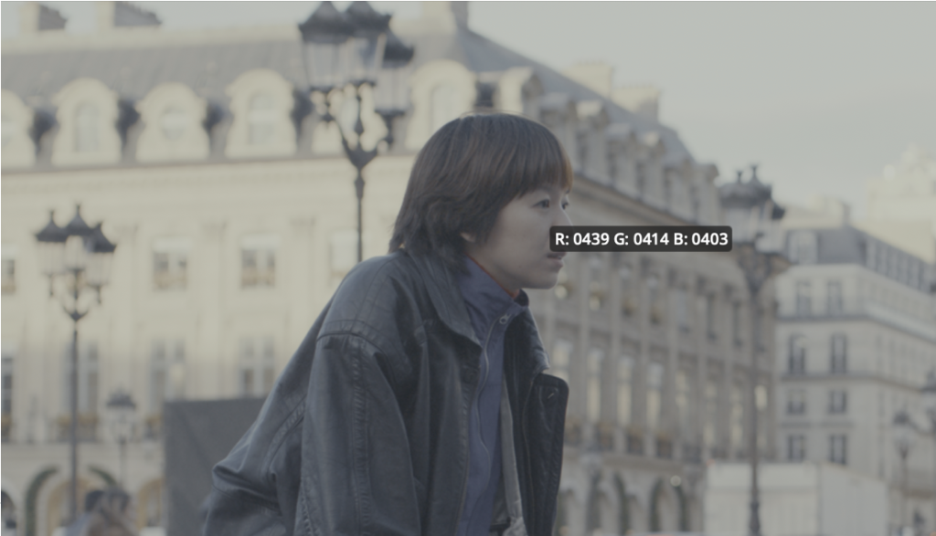
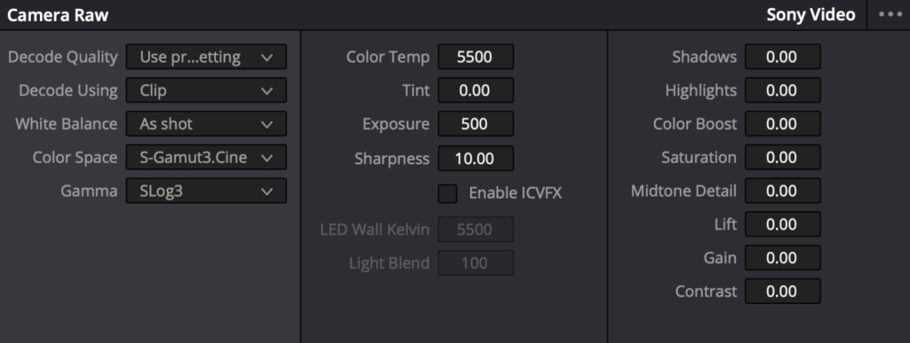
One thing that’s obvious to anyone who has worked with RAW footage—yet still striking—is just how many options some RAW module offers for adjustment: white balance, tint, exposure, and so on. Changing these parameters drastically alters the resulting RGB values, despite the fact that only one image was ever formed by the lens on the camera sensor.
To understand what these RGB values really mean, and how RAW development parameters influence them, we’ll open the black box and explore how a camera produces these values from its sensor output, given a certain set of RAW development parameters.
How the RAW image data are obtained ?
What is really happening under the hood between the formation of the image on the sensor and the output of the RAW processing module is kept as an industrial secret by the high-end cinema camera manufacturers. Still, we can infer what is going on with a bunch of clues from different sources.
Useful sources of information include : documentation from CMOS sensors manufacturers, open source projects and digital still camera RAW files. Indeed, digital still camera RAWs can be encoded in DNG (Digital Negative1) which is an open format, meaning that we can directly read the RAW pixel data without most of the processing and have access to a lot of meaningful metadata. Other information can be gathered by vendor-supplied technical documentation and analysis of the behaviour of raw processing modules.
The digital sensor response
Our story begins when the image is formed by the lens on the sensor surface and integrated by the sensor during a certain time, called the exposure time and generally around 1/50 s for cinema.
The sensor can be thought of as an array of little photo-sensitive cells, called photo-sites.
The amount of light integrated by a photo-site during the exposure time is simply called the exposure. The exposure for a given photo-site depends on the aperture of the lens, the exposure time, the amount of flare and of course the subject itself. The brightest parts of the subject produce high exposure while darker parts produce lower exposure.
We can think of a photosite as a tiny well that collects photons. The well is ‘open’ for the duration of the exposure; once the shutter closes, the sensor measures the accumulated charge and generates a voltage proportional to the photon count. While simplified, this model accurately reflects the underlying physics.
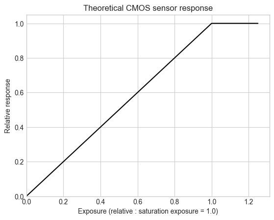
The sensor response to exposure is linear, meaning that doubling the amount of light on the sensor doubles the sensor response. This is true until the photosite saturates.
Saturation happens when the cavity gets filled up, subsequent photons cannot enter and so they have no impact on the sensor’s response. When the exposure exceeds the saturation exposure, the sensor cannot differentiate different exposure levels anymore resulting on an artefact called clipping.
The signal from the sensor is then sent through some post treatments circuits. High end camera generally have two different electronical circuits : one for low light levels and one for high light levels. Some manufacturers like ARRI with the ALEV 4 sensor choose to merge the output of two circuits into a single high dynamic range image, while some other like SONY with the Venice cameras chooses to let the user switch between two outputs, called “ISO base”. Of course the exact nature of those circuits are industrial secrets.
In the end the result of this process is generally a linear response to light within a certain exposure range, called the dynamic range, limited by noise level in the low lights and saturation in the highlight. In practice the relation between the scene and the response is never absolutely linear, principally because of flare.
Flare is a general illumination on the sensor cause by reflection within the lens and the interior of the body of the camera. If you’ve already looked at a digital sensor, you can see that it is shiny and reflects a lot of light. Flare is inevitable and is an important characteristic of image reproduction workflows as it reduces contrasts in the low lights.
RGB filters and spectral sensitivity
For now we only considered the response of the sensor to the amount of light independently from it’s colour. Digital camera’s sensors do analyse the colours of the image formed by the lens using an array of coloured filters. The most common layout, using three filters, Red, Green and Blue arranged in a 2-by-2 pattern, is called the Bayer filter.
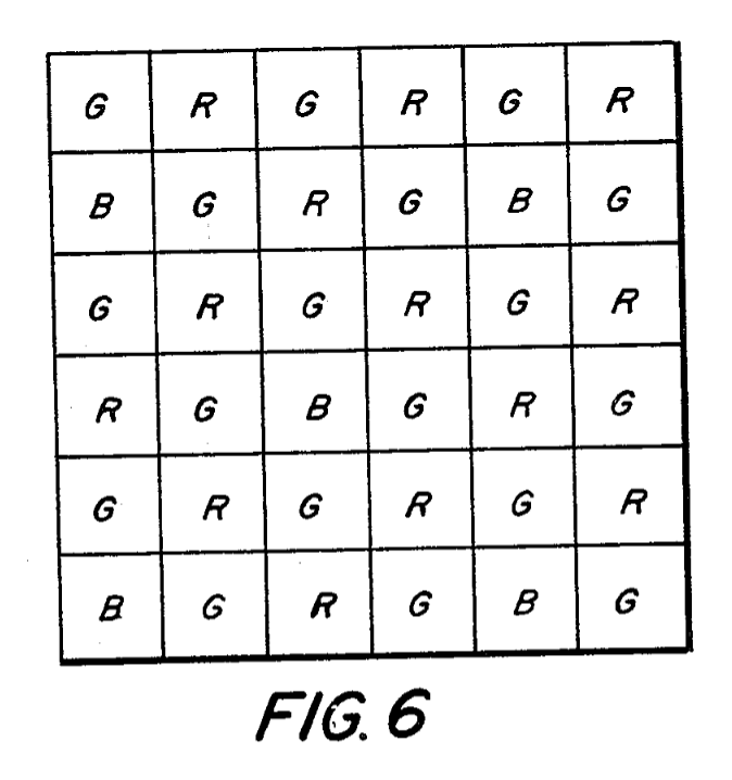
It is well known that each photo-site carries only the information for one of the three RGB channels and that the other channels are interpolated during a process called demosaicing or debayerisation. This process is very interesting, yet off-topic for today’s article.
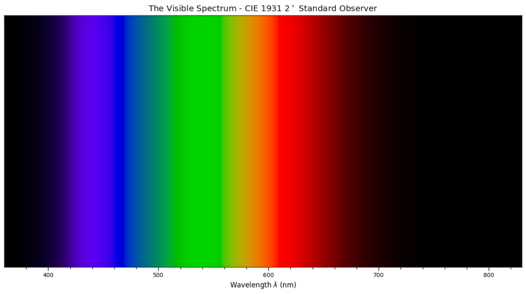
The set of RGB filter chosen by the manufacturer alongside the natural properties of the bare photo-sites define the sensor’s spectral sensitivity. The spectral sensitivity can be represented by a graph, with wavelength of the light on the x-axis and relative response of each RGB channels on the y-axis. If you are not familiar with the visible spectrum, here is a graduated and coloured representation, please note that the colours are not accurate because no screen can reproduce pure wavelengths.
On the graph below you can see the typical spectral sensitivity of a digital camera. You can see that the filters do overlap a lot. It is necessary in order to allow for a fine colour analysis. As an example, let’s think of two different shades of red, of course they will both produce a red signal, but if they only produce a response in the red channel it won’t be possible to differentiate one from another, the overlapping of the filters prevents that, in the example below you can see that no spectrum can produce a response only on one channel.
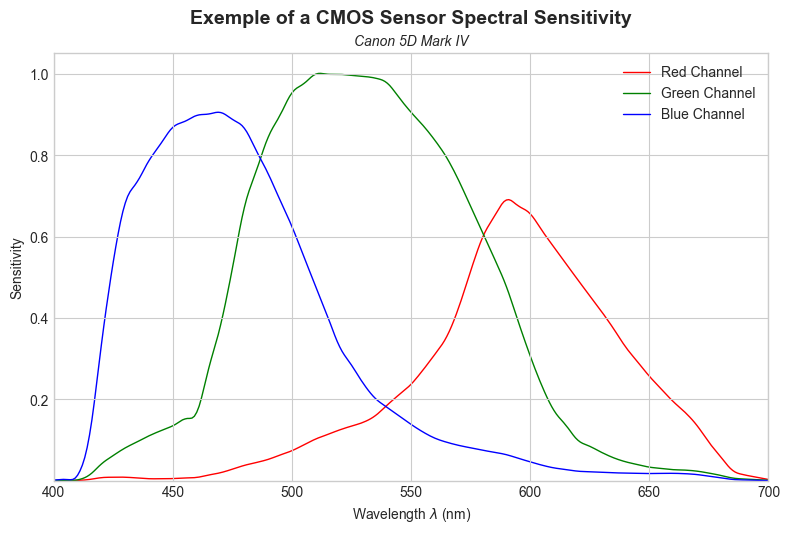
Another thing to look at is the imbalance between the sensitivities in the different channels. We can see that the red channel is less sensitive than the blue channel, meaning that in order to perform the white balance with a Daylight illuminant which contains more blue than red light, we’ll need to amplify the red channel a lot, potentially adding more noise. Whereas for a tungsten illuminant (with more red than blue) we would need less amplification. This property explains why the dynamic range and noise characteristic of a camera depends on the colour temperature of the illuminant of the scene!
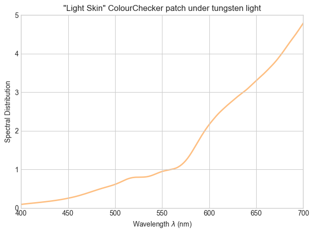
These spectral sensitivities will define the analysis of the red, green and blue component of the spectrum of the incoming light from the scene. Let’s take, as an example, the colour of the light skin patch of a colour checker, illuminated by the A illuminant (corresponding to tungsten light, around 2856K).
You can find the spectrum of this patch under tungsten lighting below. As you can see there is a lot of energy in the red side of the spectrum as the tungsten light is really warm in colour:
Here is the same spectrum weighted by the spectral sensitivity of the CMOS sensor :
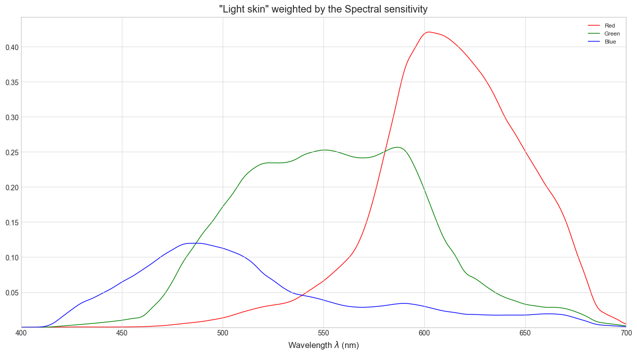
As you can see the filters allow the camera to analyse the fact that there is a lot of energy in red and not a lot of energy in blue. In this example, the resulting RGB values would be R = 0.31, G = 0.28 and B = 0.11. The scaling of those values of course depends on the exposure, if we would open on stop, it would lead to values R=0.62, G=0.56 and B=0.22 and so on. But the ratio between R, G and B stays the same.
Black Box Encoding
It is interesting to note that, for cinema camera, we don’t have access to the way the RAW data are encoded in the RAW files and each manufacturer uses a different approach. Sony and RED say that they use linear 16bit encoding while ARRI says they are using a 13bit log. There is no way to verify those statements as the raw format used by high-end camera are proprietary.
It is important to understand that the encoding of the data in the raw file is not the same as the camera colour space and log encoding. For instance the choice between Slog2 and Slog3 for a Sony camera is a RAW processing choice and is only carried by a metadata written in the raw file.
In the same fashion, as we will discuss later, RAW data are generally encoded as a response under Red, Green and Blue filters and not as RGB values related to a certain defined colour space like Sgamut3 or Sgamut3.cine, those are also metadata.
How does the RAW processing step produces RGB values from raw RGB data?
As we said before we will only analyse the colour side of raw processing and not the spatial one. So we are back to our image after the demosaicing step. Each pixel is now comprised of three values, Red, Green and Blue, linearly related to the amount of light captured by the sensor under his specific set of RGB filters.
Those value are in the black box. In order to produce an output in the software, the image needs to go through the manufacturer raw processing module given a certain set of metadata, by default the one set by the operator while shooting.
The RGB output of the raw processing module is scene-referred data. We will discuss later of the full definition of scene-referred but for now let’s look at the conversion from raw RGB to scene-referred RGB.
Note that the order and exact nature of the operations can vary depending on the camera manufacturer but the approach described below is very common. It is also the approach generally taken to process RAW from still camera DNG files.
White balance scaling
Given a RGB colour space, the chromaticity that corresponds to three identical RGB values is called the white point chromaticity.
The native white point of the sensor is generally not really interesting and does not necessarily corresponds to real-life illuminants, for instance a lot of digital still cameras have a more transparent green filter, so it would need a magenta illuminant to a achieve equality between Red, Green and Blue. Anyway, as our eyes adapt to viewing conditions, we want to be able to choose what is white in our image.
So the first step of our RAW processing journey is to scale the RGB value in order to assign equal RGB values to the neutral zones of our scene. This step is called white balance and is pretty simple.
Following our precedent example, the “light skin” patch illuminated by 2855K tungsten light, with RAW RGB value of (0.31, 0.28, 0.11).
A RAW processing module knows that a white patch under the same illuminant would result in RGB values of (0.80, 1.0, 0.46). Thus, it will scale the values by (1/0.80, 1.0, 1/0.46) in order to get RGB values of (1, 1, 1) for the white patch. The same scaling would give for the light skin patch RGB values of (0.39, 0.28, 0.24). Both Red and Blue values are increased, reflecting the fact that the sensor is more sensitive to green and thus needs amplification of the Red and Blue channel in order to obtain a neutral image.
Colour Mapping to CIE XYZ
Now we’ve got our image comprised of RGB values correctly scaled depending of the illuminant of the scene. But as we said before, those RGB values correspond to the amount of light analysed under a certain set of RGB filters that vary from a camera to another. We have no idea what is the real colour of an object in the scene given this RGB values. We need to express those RGB values against a reference of some kind.
The most broadly used system for colour measurement is called the “CIE 1931 2° Standard Colorimetric Observer” or sometimes simply “CIE XYZ”. It is defined by a set of three colour matching function.
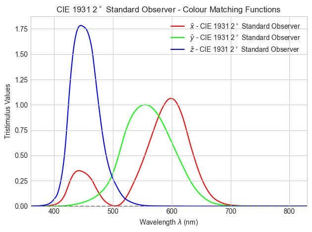
We can think about those colour matching functions as camera filters. An ideal colorimeter (some screen calibration probe for instance) is a device that measures light through those three specific filters and output the tri-stimulus values X, Y and Z.
By definition two different spectrum with the same XYZ values should yield the same visual appearance no matter their spectral power distribution. This is really interesting for our use case. If we knew the XYZ value corresponding to the RAW RGB values, we could reproduce scene colours on a screen by displaying the same XYZ values.
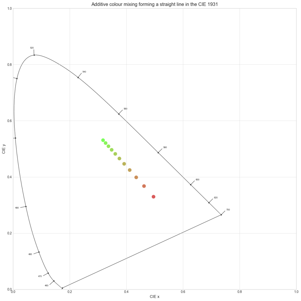
You certainly already have encountered the CIE 1931 xy chromaticity diagram, which is a 2D representation of the XYZ colour space, each point on the diagram represents the chromaticity of a given colour. Two colour with the same chromaticity coordinate on this diagram are only differentiated by their energy level (and so their Luminance).
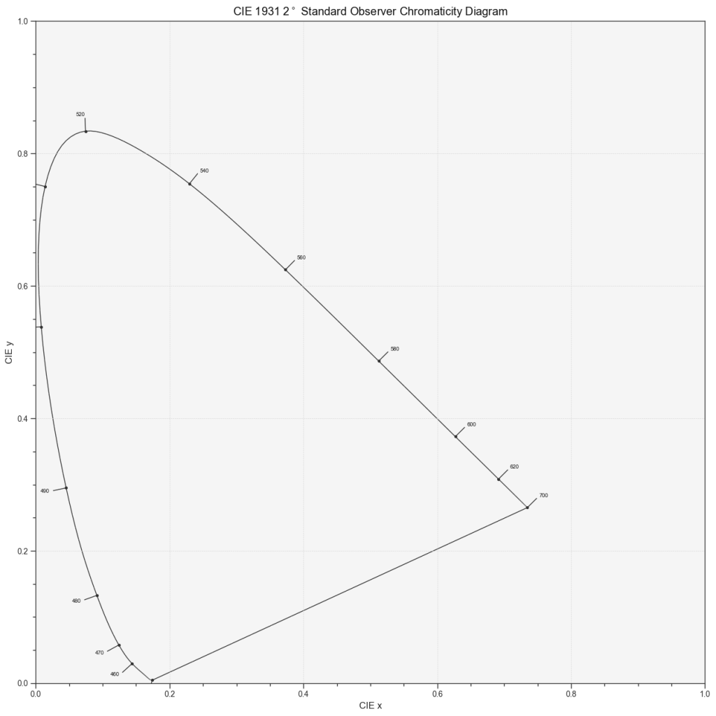
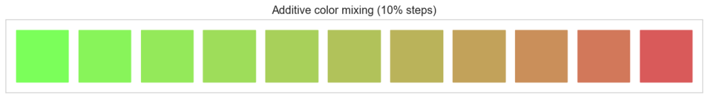
In this diagram, the chromaticity of an additive mixture of two colours lies on the straight line connecting their chromaticity coordinates.
The horseshoe looking line on this diagram is called the spectrum locus, corresponding to the chromaticity coordinates of the monochromatic lights. All the colours are a mix of monochromatic wavelengths between 380nm and 780nm, thus they are all situated inside the shape formed by the spectrum locus and the straight line between the 380nm and 780nm monochromatic lights, called the line of purples.
Everything plotted on this diagram is defined in relation to the CIE 1931 2° XYZ Standard Observer.
In order to be able to determine what actual colour corresponds to some RAW RGB values, the manufacturer must design a transformation from RAW RGB to XYZ. This transformation happens in the black box. The simplest form for this mapping is a linear map that can be represented by a 3×3 matrix:
If you are not familiar with this notation, it just another way of writing:
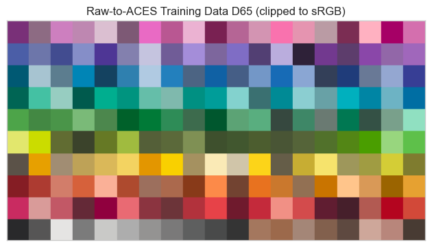
Linear map are really basic, each X, Y and Z are just some proportion of R, G and B. In order to design such transformation the manufacturer must compare the RAW RGB output of its camera with the corresponding XYZ data for a large amount of colour samples and find the best matrix. An example dataset for this purpose is the ones given by the Academy of Motion Picture Arts and Sciences3 :
Even if the value are scaled in accordance with the white point it is necessary to optimise the matrix depending on the colour temperature, so the white balance metadata has an impact on the RAW to XYZ matrix too. It is generally sufficient to generate two matrices, one for daylight and one for tungsten. Transforms for an in-between illuminant are generated by interpolating between the two matrices.
This transformation maps RAW RGB values to the corresponding colours in the XYZ models that reflect the human perception of colour.
As a linear map is a very simple transformation, the mapping is far from perfect. You can see an illustration of the resulting approximations in the example plot below. The main reason is that spectral analysis (by the XYZ colour matching function or camera filters) are loosing a lot of information mapping a full spectrum to just three values, as a result the relationship between two different spectral analysis is deeply non-linear. However, the linearity of the transform has advantages we will discuss later in this article. Some manufacturers may also use non-linear transforms to achieve better accuracy, but they must be careful as non-linear transforms can easily create artefacts if not done correctly. It is interesting to note that there is no prefect mapping from raw RGB to XYZ as a spectrum that yields identical raw RGB values can correspond to different XYZ values.
The correspondence with the XYZ model is not the only thing that happens during this stage of the RAW processing. The colour matrix is also responsible of the mapping the RAW RGB scaled white point (R=G=B) to a certain chromaticity, which will become the chromaticity of the white point of the encoding space. Generally this white point is D65, which corresponds to daylight with a correlated colour temperature around 6500K as it is the white point’s chromaticity of most displays.
The output of this process is the scene represented in XYZ as if it was seen under a D65 illuminant. This is great because the data carry both reference to the actual colour of the scene in a standardised system and the white balance intentions.
As discussed above, nowadays camera manufacturers use different matrices depending on the RGB ratios to be able to perform a more precise mapping. This operation is locally linear but globally non-linear, and can cause issues for tools that relies on the linearity of additive mixing (see below).
Exposure
As we discussed earlier the sensor has a linear response to light, and more importantly, given an “ISO base” for dual-ISO camera, it has only one response to light. However, modern cameras can be used within a wide range of exposure due to their relatively high dynamic ranges. The ISO, or EI for Exposure Index, metadata is carrying the information of the exposure level the operator chose to work with on set.
There is a direct relation between the Exposure Index and the average exposure level defined in the standard ISO 12232:20194 :
Where is the Exposure Index and is the average exposure on the image plane.
It means that when you are setting your camera to a certain EI/ISO value, your are effectively telling the RAW processing module that you are working with a certain amount of light on average.
Statistically speaking, it is admitted that, considering an average scene, the average luminance on the image plane corresponds to the light reflected by a 18% grey card in the same lighting conditions. But camera manufacturers are free to interpret the ISO standard as they see fit, as it is just a recommendation for digital cameras, whereas for films there is a mandatory procedure to follow in order to assess an ISO sensitivity.
The RAW processing module knows the RAW signal level corresponding to each exposure level and is able to encode the 18% grey value to a certain code value. This value will then be mapped to linear digital value 0.18. It is generally considered as the reference point for exposure.
This mapping can be performed during the encoding process, for instance let’s look at this graph from ARRI LogC4 documentation5 as an illustration:
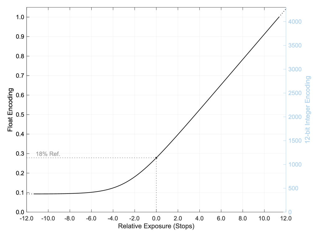
We can see that the 18% grey corresponding to 0.0 on the relative exposure scale is encoded to a certain code value, 0.278 on this graph. So when we decode we will map 0.278 to 0.18 in linear. The decoding will be perform by using the inverse of the encoding curve.
In order to achieve the mapping in the encoding stage, what ARRI is effectively doing is mapping the signal level corresponding to the 18% grey exposure, depending on the exposure index chosen by the operator, to the defined code value. In LogC4 the mapping is done through the usage of a certain encoding function, mapping the raw value to a given encoded value depending on the E.I. setting:
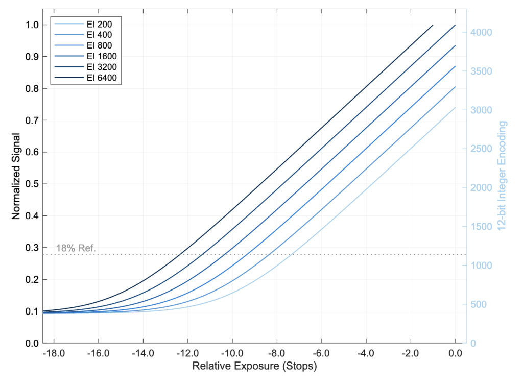
As you can see, in this case the 0.0 is the clipping point of the sensor, and the choice of an E.I. results on a different position for the neutral grey on the relative exposure scale. We can understand the choice of an E.I. as positioning the neutral grey on the dynamic range of the camera.
Other manufacturers don’t give such a comprehensive documentation, but they all provide a certain code value corresponding to the neutral grey, and an encoding function relative to this peculiar point.
This neutral grey mapping allows the scene-referred data to carry the exposure choice of the operator.
Encoding
We already talk a bit about encoding in the previous section because the mapping of the neutral grey can be (and is usually) done during encoding. But a question arises, why do we need to encode with a log curve ? The response of the sensor being linear, why don’t we keep things linear with a simple gain for the neutral grey ?
The justification for the usage of log-like functions to encode image data comes from optimising the encoding on limited bit-depth.
Our perception of the intensity of a visual stimulus can be approximated by a logarithmic progression. This result is called the Webner-Feschner law. Actually this law is a good approximation for a lot of perceptual phenomenon like tactile and sound perception!
A useful thought experiment to understand what it means is to imagine a dark room. If I light up a lamp in the room, the perceived brightness in the room increases a lot, if I light up a second one, the perceived brightness still increases, but a bit less. As you light up more and more lamp the perceived effect of lighting up a single lamp is less and less important. This is exactly the definition of a logarithmic progression.
There are better models than simple logarithmic function to describe the human quantitative perception of light if we know more about the viewing conditions, but for encoding, logarithmic function also have the advantage of matching the f-stop scale. Indeed a difference of one stop (or EV) is equivalent to multiplying/dividing the amount of light by two, thus the EV/f-stop scale is a logarithmic scale with a basis of 2.
Logarithmic scales are used since the XIXth century to represent film emulsion characteristics, so when the first film scanners were designed it felt natural to encode the scanned negative using a logarithmic scale. This scale was called Cineon. Inspired by the Cineon log, digital camera manufacturers started to encode their image with a log function too.
This is convenient because when encoding on a certain bit depth, let say 10 bits, we’ve got only a fixed number of values, here 1024 values. Log encoding allows us to allow each stop approximatively the same amount of code values.
To sum up manufacturer use log-like function to optimise the encoding by allowing roughly the same amount of code values to each f-stops. Some manufacturers propose multiple log encoding curves which differs in the amount of code values they allow to different f-stops. In the end it is important to notice that, as stated before, within the RAW file the choice of an encoding curve for the scene-referred RGB data is just a metadata.
Another side of the encoding is the choice of an RGB colour space.
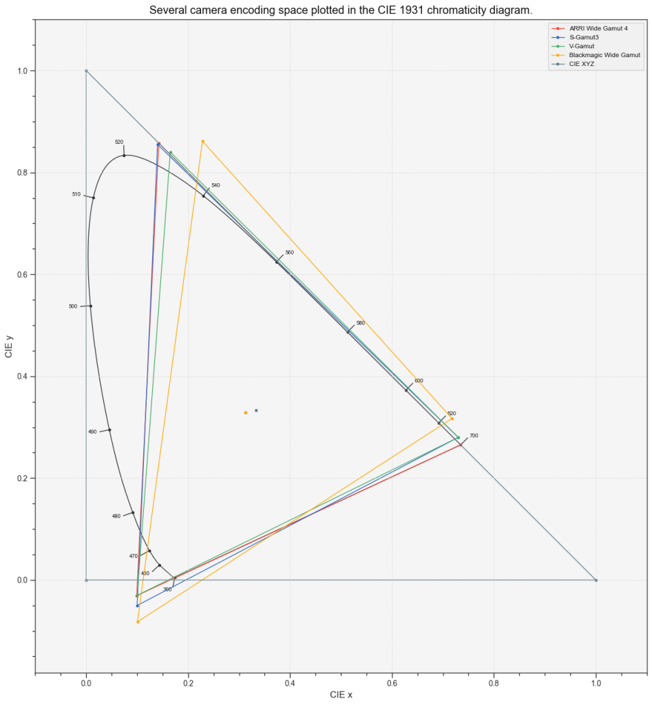
As you can see below the XYZ colour space is very big, including colours that no displays would ever be able to reproduce, and even code values that represent chromaticity points beyond the spectrum locus, referring to no actual colours present in a real scene. Moreover, colour grading tools are not optimised for the XYZ colour spaces as we will discuss below.
Converting the XYZ data to the RGB colour space is really straight forward as the Red, Green and Blue primaries are expressed in the XYZ system. You can see below the positioning of the camera encoding spaces of most camera.
There is an important difference we will discuss in the next section between encoding in RGB camera space within a colour grading software and exporting the encoded data in a ProRes (or in another file type that doesn’t support float encoding). As the later is clipping the values outside of the (0-1) range.
In the end of the RAW processing step, we obtain log-encoded RGB data corresponding to the colours of scene with a given white point assumed (generally D65).
When talking about an encoding colour space, we are generally considering an association of a colour space and an encoding function.
For now we will write them with the following syntax : colour space/encoding function, i.e. REDWideGamut/REDLog3G10.
The Scene referred state
Does encoding matters ?
While reading the last section, you might have asked yourselves, how do I choose the encoding space if there is multiple ones ? Which log is the best ? Is a bigger colour space better ?
To answer those question we need to consider two different situations : float encoding and unsigned-integer encoding.
Within a colour grading software all the image data are encoded as floating point numbers, either on 16 or 32bits, meaning that the data can be negative and can go beyond 1. In this situation, going from a bigger colour space to a smaller colour space is non-destructive.
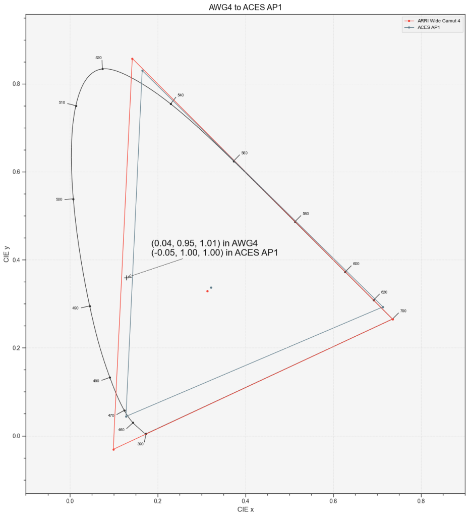
As you can see in the diagram above, if you’re converting ArriWideGamut 4 to the slightly smaller ACES AP1 gamut (the colour space of ACEScc, ACEScg and ACEScct) you get negative values but you are not clipping any information.
In the same fashion, when working in float, changing the log-like encoding function or converting to linear are non-destructive transformations.
In the other hand, if you encode scene-referred data to a certain format that requires a conversion to unsigned integers (positive integers) you won’t be carrying negatives. But this happens only if you are exporting your scene-referred data to a format like ProRes or DPX and to be totally fair as the scene-referred colour spaces are all bigger than the display colour spaces, if done correctly, the range 0-1 of any scene referred colour space is sufficient to encode all the meaningful colours for display.
Unsigned integer format are used to be able to work with lower bit-depth (10-12bits) in order to save file size. Low bit depth implies that the data should be encoded in log when working with such formats.
If you need the export scene-referred data while preserving negative values you can use the OpenEXR6 format that supports float encoding.
Generally speaking you would want to stay in a float encoding context until mastering. In this case it is a good idea to encode all the scene-referred data that come from multiple cameras or even computer generated scene to a single colour space where the grading would take place.
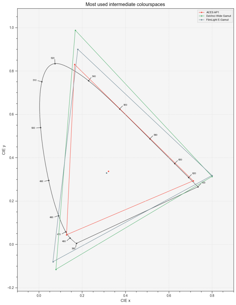
This colour space is often called intermediate colour space, the most commons are ACEScct/AP1, DaVinciIntermediate/DaVinciWideGamut and E-Gamut/T-log. But you can also use any camera scene-referred space as an intermediate, nothing stops you from converting all your inputs to REDWideGamut/Log3G10 or AWG4/LogC4. And as we said before those conversion are non-destructive as long as you stay within the colour-grading software.
Colour space and log encoding matter when it comes to using colour grading tools. But it’s not necessarily the bigger the better. It really depends on the software and the tools used, as some software/tools are colour space aware and will work identically no matter the encoding chosen. Some tools on the other end, do not adapt to the colour space and work always in the same way no matter the context, it is the case with legacy tools, designed in the film era to work with Cineon log encode images, like lift-gamma-gain for instance.
So what is scene referred ?
The CIE International Lighting Vocabulary defines the scene-referred sate as such7 :
scene-referred image state
image state associated with image data that represents estimates of the colour space coordinates of the elements of a scene.
This minimal definition, alongside with the notes you can find on the link, are not really enough to cover the way we are working with scene-referred data within cinema productions.
As you may have already realised since the beginning of this article I talked a lot about image and colours but not shown any. It is because the scene-referred state is an ambiguous state as it cannot be viewed as is. It is an unfinished image state and that carries both absolute properties of the scene and rendering intents.
Before we start grading, the scene-referred data coming from the raw processing module carries minimal rendering intents, exposure and white balance to the least. Because of the mostly linear nature of the raw processing transforms, it generally preserve the linearity of additive mixing discussed before : the chromaticity of an additive mixture of two colours lies on the straight line connecting their chromaticity coordinates.
This is important because when zones of the image are blurred, as blur acts like an additive mixing. With mostly linear transforms, the chromaticity path of the blur is preserved as a straight line. Keying tools, and interpolation tools use this property to operate correctly, so it is important to apply them (or the selection in case of a keying tool) to an image state that preserves this linearity.
It is also important to remember that the colour mapping tries to map the output of the sensor two the actual colours of the scene expressed in relation to the CIE 1931 Standard Observer XYZ system. So at this stage the scene-referred data bear a somewhat accurate relation to the actual colours of the scene.
To sum up when we consider the scene-referred state at the output of the raw processing, it carries a lot of informations about the actual scene, keeping the linearity and achieving a some kind of colour accuracy, and as said before carrying exposure and white point rendering intents.
But as we are grading in scene-referred, we are modifying the data in non-linear ways and altering the colours depending on our rendering intents. This is a good thing as grading in a scene-referred space allows us to make modifications independently of our display space.
In the end of the colour grading operations, before the DRT, the scene-referred data carry a lot of the rendering intents and is generally very far from the actual scene. But it is not yet an image, as it has only colour data but no actual colours to display and no viewing conditions. The scene-referred data don’t represent fixed colour appearances for the colours of the image, the actual colours will also depend on the display and the chosen Display Rendering Transform.
To sum up the scene-referred state is an ambiguous pre-image state that carries colour properties of the recorded scene altered following certain aesthetic rendering intents.
Look Development
Conceptually, we can define a colour look as a set of aesthetically chosen colour rendering rules that can be applied to a whole film or scene(s).
An example of such rule can be :
The lowlights are tinted in blue.
The red should darken as it increases in saturation.
The yellow is slightly orange.
The skin should appear a little warmer than natural.
The discrepancy between slightly yellow and slightly cyan greens is increased.
And so on…
You can see examples of those rules in application by watching the building the look series on the Youtube channel of HAL Picture.
In order to form a look, this set of rules should not be aimed at correcting a shot specific issue.
Practically the look will be apply in scene-referred, within the colour grading software, using a look development tool like Diachromie. The reason why look development tools like Diachromie work in a scene referred state is to be able to apply those rules on any display easily. We will discuss this process in depth in the upcoming articles of this series.
It is important that the look is the last scene-referred operation before the DRT. Indeed if you want to apply a rule like “The saturation of the green doesn’t exceed a certain threshold”, you can’t grade after the look because you could saturate the green and thus breaking the consistency.
Bonus : About Gamut
You may have noticed that I refrained myself from using the term gamut interchangeably with colour space. There is a good reason for that. Let’s look at the definition of gamut on the ILV8 :
colour gamut
volume, area, or solid in a colour space, consisting of all those colours that are either :
(a) present in a specific scene, artwork, photograph, photomechanical, or other reproduction;
or
(b) capable of being created using a particular output device and/or medium
The item (a) doesn’t apply to camera colour spaces, as it refers to a peculiar situation of image reproduction and is not a property of a device. The item (b) is describing a property of an output device. A camera doesn’t directly reproduce colours and as we said before a camera colour space is capable of encoding all the visible colours when unbound (negative and above 1) values are possible. And it is the case when we are working within the colour grading software.
Like discussed before, encoding in a scene-referred RGB colour space is just another way of writing XYZ coordinates. In mathematical terms we call this a change of basis.
So encoding into a scene-referred colour spaces doesn’t define a certain gamut. Some colours will be encoded on negative values, but this is just representation, you can encode any XYZ value, so any colours, in a scene-referred colour space. Defining a gamut implies that there is a limitation in the set of colours that can be represented.
If you decide that you will limit the range, by forbidding negative values or values above one for a specific need, scene-referred colours spaces can become limiting gamuts. In the sense of this is not possible to encode colours lying outside of the space formed by the chosen range. This can be done in order to optimise the behaviour of certain colour tools, to apply a LUT, or to encode the scene-referred data in a certain file format.
Scene-referred colour spaces taken as gamuts are usually bigger than all display colour spaces, so the operation of limiting the gamut to a certain scene-referred space, if done correctly, won’t limit the output colour palette.
That’s all for now but gamut mapping is a quite complex topic and might be the subject of another article !
What’s Next ?
The second article of this series, about display characteristics will be shorter. We will go through an in-depth tour of the display colour spaces, display encoding and viewing conditions.
If you have any questions or remarks about this article, feel free to e-mail me at : antoine.mayet@hal-picture.com
- https://helpx.adobe.com/camera-raw/digital-negative.html ↩︎
- https://patents.google.com/patent/US3971065A/en ↩︎
- https://github.com/AcademySoftwareFoundation/rawtoaces ↩︎
- https://www.iso.org/standard/73758.html ↩︎
- https://www.arri.com/resource/blob/278790/dc29f7399c1dc9553d329e27f1409a89/2022-05-arri-logc4-specification-data.pdf ↩︎
- https://openexr.com/en/latest/ ↩︎
- https://cie.co.at/eilvterm/17-32-054 ↩︎
- https://cie.co.at/eilvterm/17-32-007 ↩︎